Memory Architecture in Enterprise Data Center Solutions

Modern enterprise data centers are the backbone of digital operations, hosting everything from critical business applications to vast data analytics platforms. The efficiency of these systems is intrinsically linked to how memory is managed at every level, from the hardware itself to the running applications. Understanding this hierarchy is paramount for optimizing performance and ensuring system stability.

High-Performance Computing and Enterprise Data Center Solutions

High-Performance Computing (HPC) environments within enterprise data centers are constantly pushing the boundaries of what’s possible. These systems demand rapid access to massive datasets and the ability to execute complex computations with minimal latency. Traditional memory architectures can quickly become a bottleneck, limiting scalability and overall performance.

To address these challenges, innovative approaches are emerging. For instance, advanced software-defined memory solutions are redefining how memory resources are pooled, allocated, and managed across an entire data center. These solutions enable dynamic allocation of memory, allowing resources to be provisioned and de-provisioned on demand, much like software-defined networking or storage. This flexibility is crucial for enterprise-grade scalability, where workloads can fluctuate dramatically, and efficient resource utilization directly impacts operational costs and application responsiveness. By abstracting memory from specific hardware, organizations can achieve greater agility, optimize resource distribution, and enhance the overall performance of their HPC and general-purpose workloads.

Memory Hierarchy and Hardware Bottlenecks

The performance of any computing system, especially in an enterprise context, is heavily influenced by its memory hierarchy. This hierarchy is a structured arrangement of storage devices, ordered by speed, cost, and capacity. At the top are the fastest, smallest, and most expensive components, while at the bottom are the slowest, largest, and cheapest.

1. Registers: These are tiny storage locations directly within the CPU, offering the fastest access speeds. They hold data that the CPU is actively processing.
2. CPU Cache (L1, L2, L3): Located on or very close to the CPU, caches store frequently accessed data and instructions. L1 cache is the fastest and smallest, followed by L2 and L3. Accessing data from cache is significantly faster than from main memory.
3. RAM (Random Access Memory): Also known as main memory, RAM is where the operating system and currently running applications store their data. While much larger than cache, it’s slower.
4. Secondary Storage (SSD/HDD): This includes Solid State Drives (SSDs) and Hard Disk Drives (HDDs). These are non-volatile, persistent storage devices used for long-term data storage. Access speeds are orders of magnitude slower than RAM, but capacity is far greater.

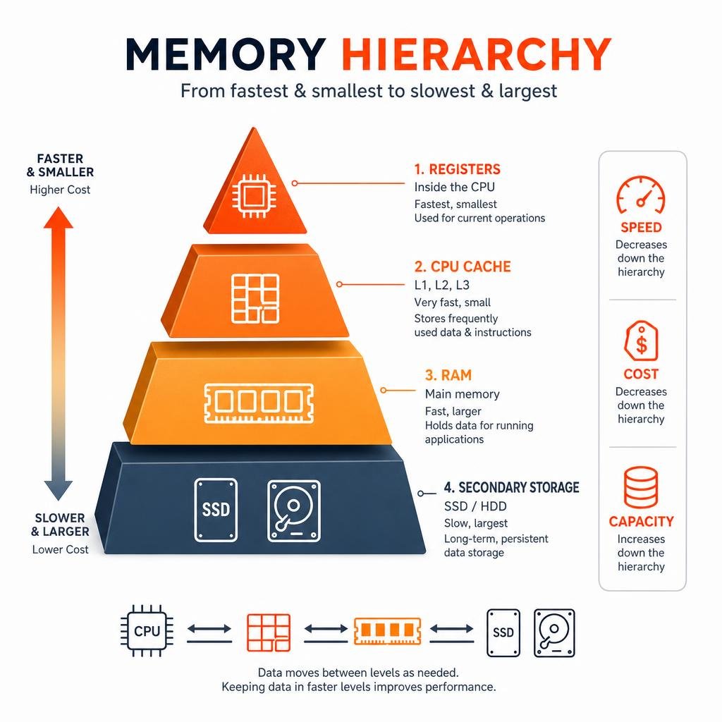
Each level of this hierarchy presents a trade-off between speed, cost, and capacity. The goal is to keep the most frequently used data in the fastest memory levels. However, the inherent latency and throughput differences between these tiers create hardware bottlenecks. When the CPU needs data that isn’t in its registers or cache, it must fetch it from slower RAM, or even worse, from secondary storage. These “cache misses” or “page faults” can significantly degrade application performance, especially in data-intensive enterprise workloads. Understanding this hierarchy is the first step toward effective application memory management, as it dictates the fundamental performance characteristics that software must contend with.

Operating System and Application-Level Memory Foundations

Beyond the hardware, the operating system (OS) plays a pivotal role in abstracting and managing the complex memory resources for applications. It provides a consistent interface for programs to request and use memory, while simultaneously protecting different applications from interfering with each other.

Address Spaces and Swapping in Enterprise Data Center Solutions

At the heart of OS memory management are the concepts of logical and physical address spaces.

• Logical Address Space: This is the set of addresses that a program perceives and generates. From an application’s perspective, it often has access to a large, contiguous block of memory, starting from address 0. This abstraction simplifies programming by shielding developers from the complexities of actual physical memory layout.
• Physical Address Space: This refers to the actual addresses available in the main memory (RAM) of the computer. These addresses correspond to the real hardware locations where data is stored.

The OS’s Memory Management Unit (MMU) is responsible for translating logical addresses generated by the CPU into physical addresses. This translation is crucial for several reasons, including memory protection (ensuring one process cannot access another’s memory) and allowing programs to use more memory than physically available through virtual memory techniques.

Static and Dynamic Loading/Linking: How programs are loaded and linked also significantly impacts memory use.

• Static Loading: The entire program is loaded into memory before execution begins. This can be inefficient if large portions of the code are rarely used, consuming valuable RAM unnecessarily.
• Dynamic Loading: Program routines are loaded into memory only when they are needed. This saves memory by avoiding the loading of unused routines, making it particularly beneficial for large applications with many features.
• Static Linking: All required library routines are combined directly into the executable file at compile time. This results in larger executables but fewer runtime dependencies.
• Dynamic Linking: Library routines are linked at runtime. A “stub” is used for library calls; at runtime, it checks if the routine is in memory and loads it if not. This reduces executable size and allows multiple programs to share a single copy of a library in memory, conserving resources.

Swapping: When the total memory demand of active processes exceeds the available physical RAM, the OS employs a technique called swapping. This involves moving entire processes, or parts of them, between main memory and secondary storage (e.g., SSD). If a higher-priority process needs to run and there isn’t enough free RAM, a lower-priority process might be “swapped out” to disk. When the swapped-out process is needed again, it’s “swapped in.” While essential for enabling multiprogramming and allowing more applications to run than physical memory permits, swapping introduces significant latency due to slow disk I/O, which can impact performance in enterprise applications.

Contiguous vs. Non-Contiguous Memory Allocation

The operating system must decide how to allocate physical memory to processes. Two primary approaches exist:

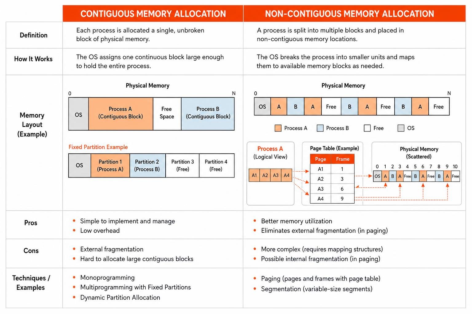
• Contiguous Memory Allocation: In this method, each process is allocated a single, unbroken block of physical memory.
• Monoprogramming: The simplest form, where memory is divided into two sections: one for the OS and one for a single user program. The OS is protected by a “fence register.”
• Multiprogramming with Fixed Partitions: Memory is divided into a fixed number of partitions, each of a fixed size. Each partition can hold one process. While simple, it can lead to inefficient memory use if processes don’t perfectly fit the partition sizes. This approach is straightforward but often suffers from fragmentation.
• Non-Contiguous Memory Allocation: To overcome the limitations of contiguous allocation, processes are allowed to reside in non-contiguous memory blocks. This flexibility helps to utilize memory more efficiently and reduces fragmentation. Paging and segmentation, discussed next, are key non-contiguous methods.

Memory Allocation Strategies (Fixed vs. Dynamic Partitions):

• Fixed Partition Allocation: As mentioned, memory is divided into fixed-size partitions. This is simpler to manage but can lead to internal fragmentation (if a process is smaller than its partition) or external fragmentation (if small free blocks are scattered).
• Dynamic Partition Allocation: Memory is divided into variable-sized partitions as needed. When a process requests memory, the OS finds a block of sufficient size. When a process terminates, its memory is returned, potentially merging with adjacent free blocks. This is more flexible but requires more complex management and can still lead to external fragmentation.

Placement Algorithms: When using dynamic partitioning, the OS needs a strategy to decide which free memory block to allocate to a new process.

• First Fit: The OS scans the list of free memory blocks and allocates the first block it finds that is large enough to satisfy the request. It’s fast but can leave small, unusable fragments at the beginning of the free list.
• Best Fit: The OS searches the entire list of free blocks and allocates the smallest block that is large enough. This strategy aims to minimize wasted space within the allocated block, potentially leading to smaller internal fragmentation. However, it can be slower due to the need to search the entire list.
• Worst Fit: The OS allocates the largest available free block. The idea is to leave a large enough remaining free block to accommodate future large requests. This can be effective in some scenarios but might also lead to rapid fragmentation of large free blocks.
• Next Fit: Similar to First Fit, but it starts searching for a suitable free block from where the last allocation left off, rather than always from the beginning. This can distribute allocations more evenly across memory but might still suffer from similar fragmentation issues as First Fit.

Paging, Segmentation, and Fragmentation Mitigation

To further enhance non-contiguous memory allocation and combat fragmentation, operating systems employ sophisticated techniques like paging and segmentation.

• Paging: This technique divides a process’s logical address space into fixed-size blocks called pages. Correspondingly, physical memory is divided into fixed-size blocks of the same size called frames. The OS maintains a page table for each process, which maps its logical pages to physical frames. This allows a process to be scattered across non-contiguous physical memory frames, eliminating external fragmentation. However, it can introduce internal fragmentation if a process’s last page doesn’t fully fill its allocated frame. The Translation Lookaside Buffer (TLB), a special hardware cache, speeds up this address translation. For enterprise systems, especially those dealing with large memory footprints, Linux’s Huge Pages (2MB or 1GB) can significantly improve performance by reducing TLB misses.
• Segmentation: Unlike paging’s fixed-size blocks, segmentation divides a program into logical units of varying sizes called segments. These segments correspond to logical divisions of a program, such as code, data, stack, or subroutines. Each segment has a name and a length. The OS uses a segment table to map these logical segments to physical memory addresses. Segmentation provides better protection and sharing at a logical level but can still suffer from external fragmentation because segments are variable-sized.

Fragmentation Mitigation:

• Internal Fragmentation: Occurs when a process is allocated more memory than it needs, leaving wasted space within the allocated block. Paging is susceptible to this. Mitigation often involves careful sizing of pages or using demand paging, where pages are loaded only when accessed.
• External Fragmentation: Occurs when free memory exists but is scattered in small, non-contiguous blocks, preventing the allocation of a larger contiguous space. Segmentation is prone to this, as are dynamic partitioning schemes.
• Compaction: A common mitigation technique for external fragmentation involves relocating existing memory blocks to coalesce all free spaces into one large, contiguous block. This is computationally expensive as it requires moving data, but it can be essential for systems needing large contiguous memory regions. Linux employs memory compaction to address this, especially for things like DMA buffers.

Stack vs. Heap Memory Allocation

Within a program’s logical address space, two primary regions are used for memory allocation: the stack and the heap.

• Stack Memory: This is a region of contiguous memory that operates as a Last-In, First-Out (LIFO) buffer. It’s primarily used for storing local variables, function parameters, and return addresses during function calls. Each time a function is called, a new “stack frame” is pushed onto the stack, containing these elements. When the function returns, its stack frame is popped off. Stack memory is managed automatically by the CPU, offering very fast allocation and deallocation. Its size is typically fixed or determined at compile time, and exceeding this limit results in a stack overflow.
• Heap Memory: This is a larger, more flexible region of memory used for dynamic memory allocation. Unlike the stack, memory on the heap is not allocated in a contiguous, LIFO manner. It’s used for storing objects whose size is not known at compile time or whose lifetime extends beyond the scope of a single function call. Examples include global variables, dynamically allocated data structures (like linked lists or trees), and objects in languages like Java or Python. Heap memory management is more complex, often involving manual intervention (in languages like C/C++) or automatic garbage collection. Improper management can lead to memory leaks or heap fragmentation.

Understanding the distinction between stack and heap is critical for developers, as it dictates how data is stored, its lifetime, and the performance implications of allocation and deallocation.

Manual vs. Automatic Memory Management

The responsibility of managing memory—allocating it when needed and releasing it when no longer required—can fall to either the programmer or an automated system.

• Manual Application Memory Management (MAMM): In languages like C and C++, developers explicitly manage memory using functions like malloc(), calloc(), realloc(), and free().
• Advantages: Offers fine-grained control over memory allocation and deallocation, potentially leading to highly optimized performance. Developers can tailor memory usage precisely to application needs.
• Disadvantages: Highly prone to errors. Common issues include memory leaks (failing to free allocated memory), dangling pointers (accessing freed memory), double frees (freeing the same memory twice), and buffer overflows. These bugs can be difficult to debug and can lead to crashes, security vulnerabilities, and unpredictable behavior. Techniques like RAII (Resource Acquisition Is Initialization) in C++ help mitigate some of these risks.
• Automatic Application Memory Management (AAMM): High-level languages like Java, Python, C#, and JavaScript employ AAMM, primarily through garbage collection (GC). The runtime environment automatically detects and reclaims memory that is no longer reachable or used by the program.
• Advantages: Simplifies development significantly by removing the burden of manual memory management from the programmer. Reduces common memory-related bugs, leading to more robust and secure applications.
• Disadvantages: Introduces overhead. Garbage collection cycles can cause pause times (also known as “stop-the-world” pauses) where application execution is temporarily halted, impacting real-time performance or user experience. The timing of GC is often non-deterministic, making performance tuning more challenging.

Garbage Collection Algorithms:

• Reference Counting: Each object maintains a count of references pointing to it. When the count drops to zero, the object is considered garbage and its memory is reclaimed. This is simple and incremental, avoiding long pauses. However, it fails to collect memory involved in circular references (where objects refer to each other but are no longer reachable from the root).
• Mark-and-Sweep: This is a two-phase algorithm.

1. Mark Phase: The GC starts from a set of “roots” (e.g., global objects, active stack variables) and traverses the object graph, marking all reachable objects.
2. Sweep Phase: The GC then scans the entire heap, reclaiming memory from all unmarked (unreachable) objects. This algorithm effectively handles circular references but can introduce longer pause times as it needs to scan the entire heap. Modern GCs often use generational approaches to optimize this, focusing on collecting short-lived objects more frequently.

The choice between MAMM and AAMM depends heavily on the application’s performance requirements, the language used, and the development team’s expertise. Enterprise systems often leverage both, with performance-critical components written in MAMM languages and higher-level business logic in AAMM languages.

Optimizing Runtime Memory in Enterprise Environments

Effective memory management is not just about understanding the underlying mechanisms; it’s about actively optimizing application behavior to ensure efficient resource utilization. In enterprise data centers, where applications run continuously and handle vast amounts of data, even small inefficiencies can accumulate into significant performance and cost overheads.

Java and Android Memory Optimization

Java and Android environments, both relying on automatic garbage collection, present unique challenges and opportunities for memory optimization.

Android Memory Management: Android’s memory management is particularly stringent due to the resource constraints of mobile devices.

• Dalvik/ART Heap: Each app process has its own constrained heap. Android’s Runtime (ART) and its predecessor Dalvik use generational garbage collection. When an app reaches its heap capacity and attempts to allocate more memory, an OutOfMemoryError can occur, leading to crashes.
• Zygote and Shared Memory: Android efficiently shares RAM pages across processes. New app processes are “forked” from the Zygote process, which pre-loads common framework code and resources, allowing multiple apps to share these memory regions. Static data (like Dalvik code, app resources, native code) is memory-mapped and shared. Dynamic RAM can also be shared using explicitly allocated shared memory regions (e.g., ashmem, gralloc).
• Proportional Set Size (PSS): Android uses PSS to measure an app’s physical memory footprint, accounting for shared memory proportionally. This gives a more accurate view of an app’s real memory impact.
• Process Lifecycle and onTrimMemory(): Android keeps non-foreground processes in a Least Recently Used (LRU) cache. When memory runs low, the system kills processes from this cache, prioritizing those that are least recently used and consuming the most memory. Apps can respond to memory pressure via the onTrimMemory() callback, releasing resources at different levels of severity (e.g., TRIM_MEMORY_UI_HIDDEN when the UI is not visible, TRIM_MEMORY_COMPLETE under critical memory pressure).

Java Optimization Best Practices: Optimizing Java applications for memory efficiency in enterprise environments involves a combination of profiling, careful coding, and architectural decisions:

• Use Memory Profilers: Tools like Eclipse Memory Analyzer or the Android Studio Profiler are indispensable for identifying memory consumption hotspots, object allocation patterns, and memory leaks.
• Optimize Data Representation: Instead of using collections of wrapper objects (e.g., ArrayList<Integer>), use primitive type arrays (int[]) where possible. For tabular data, representing it as arrays of columns rather than objects per row can save significant overhead.
• Flyweight Pattern and Caching: Employ design patterns like the Flyweight pattern to share common object states, reducing the number of objects created. Implement smart caching strategies, potentially using SoftReference or WeakReference for data that can be recreated, allowing the GC to reclaim them under memory pressure. Caching to disk for very large datasets can also be beneficial.
• Minimize Object Duplication: Ensure good normalization of the object model to avoid duplicating values. Use object pools for expensive-to-create objects.
• Avoid Unnecessary Overhead:
• Enums (Android specific): On Android, enums can consume more than twice the memory of static constants and should generally be avoided.
• Java Class/Instance Overhead: Be aware that each Java class has about 500 bytes of code overhead, and each instance has 12-16 bytes of RAM overhead. HashMap entries also add overhead (e.g., 32 bytes per entry).
• Efficient Serialization: For inter-communication, binary serialization formats like Protocol Buffers, Thrift, Avro, or MessagePack are significantly more memory-efficient than text-based formats like JSON or XML. Nano protobufs are recommended for Android client-side code.
• JVM Tuning: Fine-tune JVM command-line options, especially those related to garbage collection, to minimize pause times and optimize heap usage for specific workloads.

JavaScript Memory Management and Advanced Data Structures

JavaScript, being a high-level language, relies on automatic garbage collection. Modern JavaScript engines primarily use the mark-and-sweep algorithm, which effectively handles circular references. While developers don’t manually free memory, understanding how GC works and leveraging specific data structures can significantly aid memory management.

• WeakMaps and WeakSets: These are specialized data structures that hold keys (and values in WeakMap) “weakly.” This means that if an object used as a key in a WeakMap or WeakSet has no other strong references pointing to it, it becomes eligible for garbage collection.
• WeakMap: Keys must be objects or symbols. Values can be any type. Useful for associating metadata with objects without preventing them from being garbage collected (e.g., private data for objects, caching DOM elements).
• WeakSet: Stores only objects. Useful for tracking objects without preventing their collection (e.g., keeping track of active listeners).
• Benefit: They prevent memory leaks that can occur when objects are kept alive solely because they are keys in a regular Map or Set, especially in long-running applications or complex UIs. They are not iterable, as their contents can change unpredictably due to GC.
• WeakRefs and FinalizationRegistry: Introduced to provide more direct introspection and control over garbage collection, though their use is generally discouraged due to non-deterministic behavior.
• WeakRefs: Allow you to create a weak reference to an object. You can access the object’s value through the deref() method, but the WeakRef itself doesn’t prevent the object from being garbage collected. This is useful for building caches where items can be removed by the GC if memory is low.
• FinalizationRegistry: Allows you to register a cleanup callback function that will be executed when a registered object is garbage collected. This can be used for releasing non-memory resources (e.g., closing file handles or network connections) associated with an object after it’s been collected.
• Caution: Both WeakRefs and FinalizationRegistry have non-guaranteed runtime semantics, meaning the timing of cleanup is unpredictable. Relying on them for critical resource management can lead to subtle bugs. try...finally blocks are generally preferred for deterministic resource cleanup.

These advanced JavaScript features are powerful tools for optimizing memory usage in complex web applications and Node.js services, especially when dealing with large object graphs or long-lived processes.

Identifying and Addressing Memory Leaks

Memory leaks and inefficiencies are insidious problems that can degrade application performance over time, eventually leading to crashes or system instability. Identifying and addressing them is a critical aspect of application memory management.

What are Memory Leaks? A memory leak occurs when a program allocates memory but fails to release it when it’s no longer needed. This causes the application’s memory footprint to grow continuously, even if its actual workload remains stable. Over time, this exhausts available memory, leading to OutOfMemoryError exceptions, excessive swapping, and ultimately, application or system crashes.

Identifying Inefficiencies and Leaks:

• Memory Profilers: These are the primary tools for diagnosing memory issues. They allow developers to:
• Monitor Live Memory Usage: Track an application’s memory footprint over time, observing growth patterns.
• Analyze Object Allocations: See which objects are being created, how many, and where in the code.
• Perform Heap Dumps: Capture a snapshot of the application’s heap at a specific moment, showing all objects in memory, their sizes, and their references. Tools like Eclipse Memory Analyzer (for Java), Android Studio Profiler, Xcode Instruments (for iOS/macOS), and browser developer tools (for JavaScript) are invaluable for this.
• Diagnostic Tools:
• stressapptest: This tool can simulate high memory load conditions, helping to test how an application behaves under memory pressure. It can trigger various alerts like SIGABRT, SIGQUIT, or TRIM_MEMORY_EVENTS.
• OS-level Utilities: Commands like top, htop, ps, and vmstat (Linux/Unix), or Activity Monitor (macOS) provide insights into process memory usage, virtual memory statistics, and swap activity.
• Code Reviews: Peer reviews can often catch common memory-related anti-patterns before they become leaks.

Addressing Memory Leaks and Inefficiencies:

• Proper Resource Release: Ensure that all allocated resources (memory, file handles, network connections) are properly released when no longer needed. This often involves adhering to language-specific best practices (e.g., try-with-resources in Java, RAII in C++, event listener cleanup in JavaScript).
• Lifecycle Management: For mobile and UI applications, tie resource allocation and deallocation to the component’s lifecycle (e.g., releasing UI resources when an Android Activity is paused or destroyed).
• Optimize Data Structures: Choose memory-efficient data structures (e.g., SparseArray over HashMap for integer keys in Android).
• Minimize Object Creation: Reduce unnecessary object allocations, especially in performance-critical loops. Object pooling can help reuse objects instead of constantly creating new ones.
• Memory Limits Management: Understand and respect system-defined memory limits (e.g., Android’s heap capacity). Query available memory (getMemoryClass() in Android) and adjust application behavior accordingly. If an application consistently hits memory limits, it indicates fundamental inefficiencies that need to be addressed, rather than simply requesting more memory.

By systematically identifying and resolving memory leaks and optimizing memory usage, developers can significantly improve the stability, performance, and scalability of their enterprise applications.

Frequently Asked Questions about Enterprise Memory Management

What is memory management and why is it crucial for operating systems?

Memory management is the process of controlling and coordinating computer memory, assigning blocks to running programs, and reclaiming them when no longer used. It is absolutely crucial for operating systems because it enables efficient resource allocation, ensures data integrity by preventing programs from interfering with each other, facilitates multitasking, and allows applications to run even if their combined memory requirements exceed physical RAM through techniques like virtual memory. Without effective memory management, systems would be prone to crashes, slow performance, and security vulnerabilities.

How do paging and segmentation work as non-contiguous memory allocation methods?

Paging divides a program’s logical memory into fixed-size blocks called “pages” and physical memory into equally sized “frames.” The operating system uses a page table to map these logical pages to available physical frames, allowing a program to be scattered across non-contiguous physical memory. This eliminates external fragmentation. Segmentation divides a program into variable-sized logical units called “segments” (e.g., code, data, stack). Each segment is treated as a distinct entity. The OS uses a segment table to map these segments to physical memory. Segmentation provides logical protection and sharing but can lead to external fragmentation. Both methods allow for efficient use of physical memory by avoiding the need for large, contiguous blocks.

What are the differences between manual and automatic memory management?

The key difference lies in who is responsible for memory deallocation. In manual memory management (MAMM), the programmer explicitly allocates and frees memory using language-specific functions (e.g., malloc/free in C/C++). This offers fine-grained control and potential performance advantages but places a heavy burden on the developer, making applications susceptible to memory leaks, dangling pointers, and other hard-to-debug errors. In automatic memory management (AAMM), a runtime system (typically a garbage collector) automatically detects and reclaims memory that is no longer reachable by the program. This simplifies development, reduces memory-related bugs, and improves application robustness. However, it introduces overhead, and garbage collection cycles can cause unpredictable “pause times” that might impact performance.

Conclusion

As we’ve explored, application memory management is a multi-faceted discipline, spanning from the fundamental hardware architecture to intricate operating system mechanisms and meticulous application-level coding practices. In the context of enterprise data centers, where performance, scalability, and reliability are paramount, a deep understanding and proactive approach to memory optimization are indispensable.

From leveraging advanced concepts like paging and segmentation to mitigating fragmentation and choosing between manual and automatic memory management, every decision impacts the efficiency of your systems. Technologies such as software-defined memory solutions are transforming how we think about memory resources, offering unprecedented flexibility and scalability for modern workloads.

By embracing best practices for languages like Java and JavaScript, diligently identifying and addressing memory leaks with profiling tools, and understanding the implications of memory limits, organizations can unlock the full potential of their data center infrastructure. The journey of memory optimization is continuous, driven by evolving hardware, software, and workload demands. Mastering it today ensures that your enterprise applications are not just running, but thriving, ready to meet the challenges of tomorrow.